Distributed Communication#
MLX supports distributed communication operations that allow the computational cost of training or inference to be shared across many physical machines. At the moment we support several different communication backends introduced below.
Backend |
Description |
|---|---|
A full featured and mature distributed communications library. |
|
Ring all reduce and all gather over TCP sockets. Always available and usually faster than MPI. |
|
Low latency communication with RDMA over thunderbolt. Necessary for things like tensor parallelism. |
|
The backend of choice for CUDA environments. |
The list of all currently supported operations and their documentation can be seen in the API docs.
Getting Started#
A distributed program in MLX is as simple as:
import mlx.core as mx

world = mx.distributed.init()
x = mx.distributed.all_sum(mx.ones(10))
print(world.rank(), x)
The program above sums the array mx.ones(10) across all
distributed processes. However, when this script is run with python only
one process is launched and no distributed communication takes place. Namely,
all operations in mx.distributed are noops when the distributed group has a
size of one. This property allows us to avoid code that checks if we are in a
distributed setting similar to the one below:
import mlx.core as mx

x = ...
world = mx.distributed.init()
# No need for the check we can simply do x = mx.distributed.all_sum(x)
if world.size() > 1:
    x = mx.distributed.all_sum(x)
Running Distributed Programs#
MLX provides mlx.launch a helper script to launch distributed programs.
Continuing with our initial example we can run it on localhost with 4 processes using
$ mlx.launch -n 4 my_script.py
3 array([4, 4, 4, ..., 4, 4, 4], dtype=float32)
2 array([4, 4, 4, ..., 4, 4, 4], dtype=float32)
1 array([4, 4, 4, ..., 4, 4, 4], dtype=float32)
0 array([4, 4, 4, ..., 4, 4, 4], dtype=float32)
We can also run it on some remote hosts by providing their IPs (provided that the script exists on all hosts and they are reachable by ssh)
$ mlx.launch --hosts ip1,ip2,ip3,ip4 my_script.py
3 array([4, 4, 4, ..., 4, 4, 4], dtype=float32)
2 array([4, 4, 4, ..., 4, 4, 4], dtype=float32)
1 array([4, 4, 4, ..., 4, 4, 4], dtype=float32)
0 array([4, 4, 4, ..., 4, 4, 4], dtype=float32)
Consult the dedicated usage guide for more
information on using mlx.launch.
Selecting Backend#
You can select the backend you want to use when calling init() by passing
one of {'any', 'ring', 'jaccl', 'mpi', 'nccl'}. When passing any, MLX will try all
available backends. If they all fail then a singleton group is created.
Note
After a distributed backend is successfully initialized init() will
return the same backend if called without arguments or with backend set to
any.
The following examples aim to clarify the backend initialization logic in MLX:
# Case 1: Initialize MPI regardless if it was possible to initialize the ring backend
world = mx.distributed.init(backend="mpi")
world2 = mx.distributed.init()  # subsequent calls return the MPI backend!

# Case 2: Initialize any backend
world = mx.distributed.init(backend="any")  # equivalent to no arguments
world2 = mx.distributed.init()  # same as above

# Case 3: Initialize both backends at the same time
world_mpi = mx.distributed.init(backend="mpi")
world_ring = mx.distributed.init(backend="ring")
world_any = mx.distributed.init()  # same as MPI because it was initialized first!
Distributed Program Examples#
Getting Started with Ring#
The ring backend does not depend on any third party library so it is always
available. It uses TCP sockets so the nodes need to be reachable via a network.
As the name suggests the nodes are connected in a ring which means that rank 1
can only communicate with rank 0 and rank 2, rank 2 only with rank 1 and rank 3
and so on and so forth. As a result send() and recv() with
arbitrary sender and receiver are not supported in the ring backend.
Defining a Ring#
The easiest way to define and use a ring is via a JSON hostfile and the
mlx.launch helper script. For each node one
defines a hostname to ssh into to run commands on this node and one or more IPs
that this node will listen to for connections.
For example the hostfile below defines a 4 node ring. hostname1 will be
rank 0, hostname2 rank 1 etc.
[
    {"ssh": "hostname1", "ips": ["123.123.123.1"]},
    {"ssh": "hostname2", "ips": ["123.123.123.2"]},
    {"ssh": "hostname3", "ips": ["123.123.123.3"]},
    {"ssh": "hostname4", "ips": ["123.123.123.4"]}
]
Running mlx.launch --hostfile ring-4.json my_script.py will ssh into each
node, run the script which will listen for connections in each of the provided
IPs. Specifically, hostname1 will connect to 123.123.123.2 and accept a
connection from 123.123.123.4 and so on and so forth.
Thunderbolt Ring#
Although the ring backend can have benefits over MPI even for Ethernet, its
main purpose is to use Thunderbolt rings for higher bandwidth communication.
Setting up such thunderbolt rings can be done manually, but is a relatively
tedious process. To simplify this, we provide the utility mlx.distributed_config.
To use mlx.distributed_config your computers need to be accessible by ssh via
Ethernet or Wi-Fi. Subsequently, connect them via thunderbolt cables and then call the
utility as follows:
mlx.distributed_config --verbose --hosts host1,host2,host3,host4 --backend ring
By default the script will attempt to discover the thunderbolt ring and provide
you with the commands to configure each node as well as the hostfile.json
to use with mlx.launch. If password-less sudo is available on the nodes
then --auto-setup can be used to configure them automatically.
If you want to go through the process manually, the steps are as follows:
Disable the thunderbolt bridge interface
For the cable connecting rank
ito ranki + 1find the interfaces corresponding to that cable in nodesiandi + 1.Set up a unique subnetwork connecting the two nodes for the corresponding interfaces. For instance if the cable corresponds to
en2on nodeianden2also on nodei + 1then we may assign IPs192.168.0.1and192.168.0.2respectively to the two nodes. For more details you can see the commands prepared by the utility script.
Getting Started with JACCL#
Starting from macOS 26.2, RDMA over thunderbolt is available and enables low-latency communication between Macs with thunderbolt 5. MLX provides the JACCL backend that uses this functionality to achieve communication latency an order of magnitude lower than the ring backend.
Note
The name JACCL (pronounced Jackal) stands for Jack and Angelos’ Collective Communication Library and it is an obvious pun to Nvidia’s NCCL but also tribute to Jack Beasley who led the development of RDMA over Thunderbolt at Apple.
Enabling RDMA#
Until the feature matures, enabling RDMA over thunderbolt is slightly more involved and cannot be done remotely even with sudo. In fact, it has to be done in macOS recovery:
Open the Terminal by going to Utilities -> Terminal.
Run
rdma_ctl enable.Reboot.
To verify that you have successfully enabled Thunderbolt RDMA you can run
ibv_devices which should produce something like the following for an M3 Ultra.
~ % ibv_devices
device                 node GUID
------              ----------------
rdma_en2            8096a9d9edbaac05
rdma_en3            8196a9d9edbaac05
rdma_en5            8396a9d9edbaac05
rdma_en4            8296a9d9edbaac05
rdma_en6            8496a9d9edbaac05
rdma_en7            8596a9d9edbaac05
Defining a Mesh#
The JACCL backend supports only fully connected topologies. Namely, there needs to be a thunderbolt cable connecting all pairs of Macs directly. For example, in the following topology visualizations, the left one is valid because there is a connection from any node to any other node, while for the one on the right M3 Ultra 1 is not connected to M3 Ultra 2.
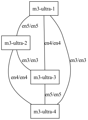
Fully connected mesh of four M3 Ultra.

Not a valid mesh (M3 Ultra 1 is not connected to M3 Ultra 2).
Similar to the ring backend, the easiest way to use JACCL with MLX is to write
a JSON hostfile that will be used by mlx.launch. The hostfile needs to contain
Hostnames to use for launching scripts via ssh
An IP for rank 0 that is reachable by all nodes
A list of rdma devices that connect each node to each other node
The following JSON defines the valid 4-node mesh from the image above.
[
    {
        "ssh": "m3-ultra-1",
        "ips": ["123.123.123.1"],
        "rdma": [null, "rdma_en5", "rdma_en4", "rdma_en3"]
    },
    {
        "ssh": "m3-ultra-2",
        "ips": [],
        "rdma": ["rdma_en5", null, "rdma_en3", "rdma_en4"]
    },
    {
        "ssh": "m3-ultra-3",
        "ips": [],
        "rdma": ["rdma_en4", "rdma_en3", null, "rdma_en5"]
    },
    {
        "ssh": "m3-ultra-4",
        "ips": [],
        "rdma": ["rdma_en3", "rdma_en4", "rdma_en5", null]
    }
]
Even though TCP/IP is not used when communicating with Thunderbolt RDMA, disabling the thunderbolt bridge is still required as well as setting up isolated local networks for each thunderbolt connection.
All of the above can be done instead via mlx.distributed_config. This helper
script will
ssh into each node
extract the thunderbolt connectivity
check for a valid mesh
provide the commands to configure each node (or run them if sudo is available)
generate the hostfile to be used with
mlx.launch
Putting It All Together#
For example launching a distributed MLX script that uses JACCL is fairly simple if the nodes are reachable via ssh and have password-less sudo.
First, connect all the thunderbolt cables. Then we can verify the connections
by using the mlx.distributed_config script to visualize them.
mlx.distributed_config --verbose \
     --hosts m3-ultra-1,m3-ultra-2,m3-ultra-3,m3-ultra-4 \
     --over thunderbolt --dot | dot -Tpng | open -f -a Preview
After making sure that everything looks right we can auto-configure the nodes
and save the hostfile to m3-ultra-jaccl.json by running:
mlx.distributed_config --verbose \
     --hosts m3-ultra-1,m3-ultra-2,m3-ultra-3,m3-ultra-4 \
     --over thunderbolt --backend jaccl \
     --auto-setup --output m3-ultra-jaccl.json
And now we are ready to run a distributed MLX script such as distributed inference of a gigantic model using MLX LM.
mlx.launch --verbose --backend jaccl --hostfile m3-ultra-jaccl.json \
     --env MLX_METAL_FAST_SYNCH=1 -- \  # <--- important
     /path/to/remote/python -m mlx_lm chat --model mlx-community/DeepSeek-R1-0528-4bit
Note
Defining the environment variable MLX_METAL_FAST_SYNCH=1 enables a
different, faster way of synchronizing between the GPU and the CPU. It is
not specific to the JACCL backend and can be used in all cases where the CPU
and GPU need to collaborate for some computation and is pretty critical for
low-latency communication since the communication is done by the CPU.
Getting Started with NCCL#
MLX on CUDA environments ships with the ability to talk to NCCL which is a high-performance collective communication library that supports both multi-gpu and multi-node setups.
For CUDA environments, NCCL is the default backend for mlx.launch and all
it takes to run a distributed job is
mlx.launch -n 8 test.py

# perfect for interactive scripts
mlx.launch -n 8 python -m mlx_lm chat --model my-model
You can also use mlx.launch to ssh to a remote node and launch a script
with the same ease
mlx.launch --hosts my-cuda-node -n 8 test.py
In many cases you may not want to use mlx.launch with the NCCL backend
because the cluster scheduler will be the one launching the processes. You can
see which environment variables need to be defined in
order for the MLX NCCL backend to be initialized correctly.
Getting Started with MPI#
MLX already comes with the ability to “talk” to MPI if it is installed
on the machine. Launching distributed MLX programs that use MPI can be done
with mpirun as expected. However, in the following examples we will be
using mlx.launch --backend mpi which takes care of some nuisances such as
setting absolute paths for the mpirun executable and the libmpi.dyld
shared library.
The simplest possible usage is the following which, assuming the minimal example in the beginning of this page, should result in:
$ mlx.launch --backend mpi -n 2 test.py
1 array([2, 2, 2, ..., 2, 2, 2], dtype=float32)
0 array([2, 2, 2, ..., 2, 2, 2], dtype=float32)
The above launches two processes on the same (local) machine and we can see
both standard output streams. The processes send the array of 1s to each other
and compute the sum which is printed. Launching with mlx.launch -n 4 ... would
print 4 etc.
Installing MPI#
MPI can be installed with Homebrew, pip, using the Anaconda package manager, or
compiled from source. Most of our testing is done using openmpi installed
with the Anaconda package manager as follows:
$ conda install conda-forge::openmpi
Installing with Homebrew or pip requires specifying the location of libmpi.dyld
so that MLX can find it and load it at runtime. This can simply be achieved by
passing the DYLD_LIBRARY_PATH environment variable to mpirun and it is
done automatically by mlx.launch. Some environments use a non-standard
library filename that can be specified using the MPI_LIBNAME environment
variable. This is automatically taken care of by mlx.launch as well.
$ mpirun -np 2 -x DYLD_LIBRARY_PATH=/opt/homebrew/lib/ -x MPI_LIBNAME=libmpi.40.dylib python test.py
$ # or simply
$ mlx.launch -n 2 test.py
Setting up Remote Hosts#
MPI can automatically connect to remote hosts and set up the communication over the network if the remote hosts can be accessed via ssh. A good checklist to debug connectivity issues is the following:
ssh hostnameworks from all machines to all machines without asking for password or host confirmationmpirunis accessible on all machines.Ensure that the
hostnameused by MPI is the one that you have configured in the.ssh/configfiles on all machines.
Tuning MPI All Reduce#
Note
For faster all reduce consider using the ring backend either with Thunderbolt connections or over Ethernet.
Configure MPI to use N tcp connections between each host to improve bandwidth
by passing --mca btl_tcp_links N.
Force MPI to use the most performant network interface by setting --mca
btl_tcp_if_include <iface> where <iface> should be the interface you want
to use.
Distributed Without mlx.launch#
None of the implementations of the distributed backends require launching with
mlx.launch. The script simply connects to each host. Starts a process per
rank and sets up the necessary environment variables before delegating to your
MLX script. See the dedicated documentation page
for more details.
For many use-cases this will be the easiest way to perform distributed
computations in MLX. However, there may be reasons that you cannot or should
not use mlx.launch. A common such case is the use of a scheduler that
starts all the processes for you on machines undetermined at the time of
scheduling the job.
Below we list the environment variables required to use each backend.
Ring#
MLX_RANK should contain a single 0-based integer that defines the rank of the process.
MLX_HOSTFILE should contain the path to a json file that contains IPs and ports for each rank to listen to, something like the following:
[
  ["123.123.1.1:5000", "123.123.1.2:5000"],
  ["123.123.2.1:5000", "123.123.2.2:5000"],
  ["123.123.3.1:5000", "123.123.3.2:5000"],
  ["123.123.4.1:5000", "123.123.4.2:5000"]
]
MLX_RING_VERBOSE is optional and if set to 1 it enables some more logging from the distributed backend.
JACCL#
MLX_RANK should contain a single 0-based integer that defines the rank of the process.
MLX_JACCL_COORDINATOR should contain the IP and port that rank 0 can listen to all the other ranks connect to in order to establish the RDMA connections.
MLX_IBV_DEVICES should contain the path to a json file that contains the ibverbs device names that connect each node to each other node, something like the following:
[
   [null, "rdma_en5", "rdma_en4", "rdma_en3"],
   ["rdma_en5", null, "rdma_en3", "rdma_en4"],
   ["rdma_en4", "rdma_en3", null, "rdma_en5"],
   ["rdma_en3", "rdma_en4", "rdma_en5", null]
]
NCCL#
MLX_RANK should contain a single 0-based integer that defines the rank of the process.
MLX_WORLD_SIZE should contain the total number of processes that will be launched.
NCCL_HOST_IP and NCCL_PORT should contain the IP and port that all hosts can connect to to establish the NCCL communication.
CUDA_VISIBLE_DEVICES should contain the local index of the gpu that corresponds to this process.
Of course any other environment variable that is used by NCCL can be set.
Tips and Tricks#
This is a small collection of tips to help you utilize better the distributed communication capabilities of MLX.
Test locally first.
You can use the pattern
mlx.launch -n2 -- my_script.pyto run a small scale test on a single node first.Batch your communication.
As described in the training example, performing a lot of small communications can hurt performance. Copy the approach of
mlx.nn.average_gradients()to gather many small communications in a single large one.Visualize the connectivity.
Use
mlx.distributed_config --hosts h1,h2,h3 --over thunderbolt --dotto visualize the connnections and make sure that the cables are connected correctly. See the JACCL section for examples.Use the debugger.
mlx.launchis meant for interactive use. It broadcasts stdin to all processes and gathers stdout from all processes. This makes usingpdba breeze.